3D tessellation of biomolecular cavities

Protocol for analyzing the ribosome exit tunnel

cryo-EM
Authors

Artem Kushner

Khanh Dao Duc

Published

August 4, 2024

Summary and Background

We present a protocol to extract the surface of a biomolecular cavity for shape analysis and molecular simulations.

We apply and illustrate the protocol on the ribosome structure, which contains a subcompartment known as the ribosome exit tunnel or “nascent polypeptide exit tunnel” (NPET). More details on the tunnel features and biological importance can be found in our previous works1,2.

The protocol was designed to refine the output obtained from MOLE software3, but can be applied to reconstruct a mesh on any general point cloud. Hence, we take the point-cloud of atom positions surrounding the tunnel as a point of departure.
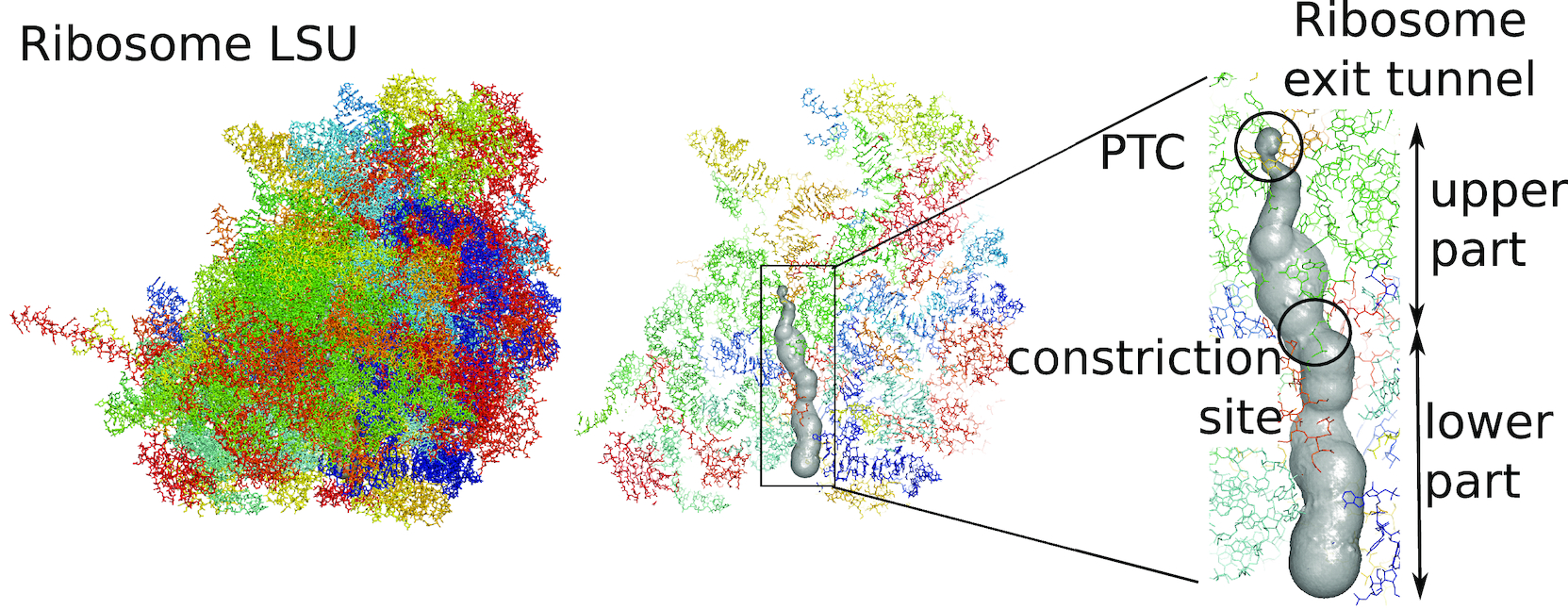
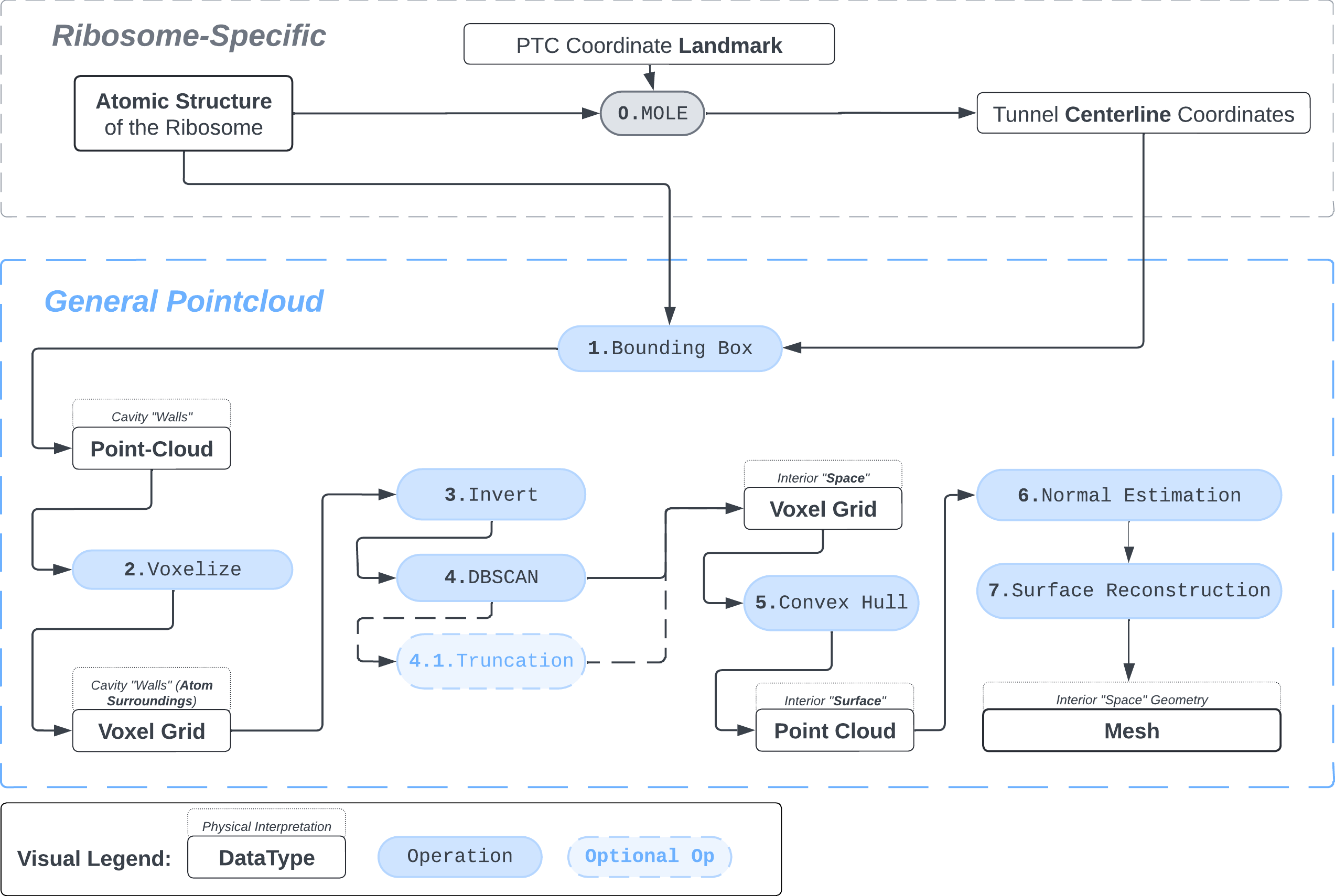
Illustration of the ribosome exit tunnel (from Dao Duc et al., NAR 2019)

1. Pointcloud Preparation: Bounding Box and Voxelization

def atompos_to_voxelized_sphere(center: np.ndarray, radius: int):
    """Make sure radius reflects the size of the underlying voxel grid"""
    x0, y0, z0 = center

    #!------ Generate indices of a voxel cube of side 2r  around the centerpoint
    x_range = slice(
        int(np.floor(x0 - radius)), 
        int(np.ceil(x0 + radius)))
    y_range = slice(
        int(np.floor(y0 - radius)), 
        int(np.ceil(y0 + radius)))
    z_range = slice(
        int(np.floor(z0 - radius)), 
        int(np.ceil(z0 + radius)))

    indices = np.indices(
        (
            x_range.stop - x_range.start,
            y_range.stop - y_range.start,
            z_range.stop - z_range.start,
        )
    )

    indices      += np.array([x_range.start,
                              y_range.start,
                              z_range.start])[:, np.newaxis, np.newaxis, np.newaxis ]
    indices       = indices.transpose(1, 2, 3, 0)
    indices_list  = list(map(tuple, indices.reshape(-1, 3)))

    #!------ Generate indices of a voxel cube of side 2r+2  around the centerpoint
    sphere_active_ix = []

    for ind in indices_list:
        x_ = ind[0]
        y_ = ind[1]
        z_ = ind[2]
        if (x_ - x0) ** 2 + (y_ - y0) ** 2 + (z_ - z0) ** 2 <= radius**2:
            sphere_active_ix.append([x_, y_, z_])

    return np.array(sphere_active_ix)
def index_grid(expanded_sphere_voxels: np.ndarray) :

    def normalize_atom_coordinates(coordinates: np.ndarray)->tuple[ np.ndarray, np.ndarray ]:
        """@param coordinates: numpy array of shape (N,3)"""

        C      = coordinates
        mean_x = np.mean(C[:, 0])
        mean_y = np.mean(C[:, 1])
        mean_z = np.mean(C[:, 2])

        Cx = C[:, 0] - mean_x
        Cy = C[:, 1] - mean_y
        Cz = C[:, 2] - mean_z
        

        [dev_x, dev_y, dev_z] = [np.min(Cx), np.min(Cy), np.min(Cz)]

        #! shift to positive quadrant
        Cx = Cx + abs(dev_x)
        Cy = Cy + abs(dev_y)
        Cz = Cz + abs(dev_z)

        rescaled_coords = np.array(list(zip(Cx, Cy, Cz)))

        return rescaled_coords, np.array([[mean_x,mean_y,mean_z], [abs( dev_x ), abs( dev_y ), abs( dev_z )]])

    normalized_sphere_cords, mean_abs_vectors = normalize_atom_coordinates(expanded_sphere_voxels)
    voxel_size = 1

    sphere_cords_quantized = np.round(np.array(normalized_sphere_cords / voxel_size) ).astype(int)
    max_values             = np.max(sphere_cords_quantized, axis=0)
    grid_dimensions        = max_values + 1
    vox_grid               = np.zeros(grid_dimensions)

    print("Dimension of the voxel grid is ", vox_grid.shape)

    vox_grid[
        sphere_cords_quantized[:, 0],
        sphere_cords_quantized[:, 1],
        sphere_cords_quantized[:, 2]  ] = 1


    return ( vox_grid, grid_dimensions, mean_abs_vectors )

Bbox: There are many ways to extract a point cloud from a larger biological structure – in this case we settle for a bounding box that bounds the space between the PTC and the NPET vestibule.

# "bounding_box_atoms.npy" is a N,3 array of atom coordinates

atom_centers = np.load("bounding_box_atoms.npy") 

Sphering: To make the representation of atoms slightly more physically-plausible we replace each atom-center coordinate with positions of voxels that fall within a sphere of radius \(R\) around the atom’s position. This is meant to represent the atom’s van der Waals radius.

One could model different types of atoms (\(N\),\(C\),\(O\),\(H\) etc.) with separate radii, but taking \(R=2\) proves a good enough compromise. The units are Angstrom and correspond to the coordinate system in which the structure of the ribosome is recorded.

voxel_spheres = np.array([ atompos_to_voxel_sphere(atom, 2) for atom in atom_centers ])

Voxelization & Inversion: Since we are interested in the “empty space” between the atoms, we need a way to capture it. To make this possible we discretize the space by projecting the (sphered) point cloud into a voxel grid and invert the grid.

# the grid is a binary 3D-array 
# with 1s where a normalized 3D-coordinate of an atom corresponds to the cell index and 0s elsewhere

# by "normalized" i mean that the atom coordinates are
# temporarily moved to the origin to decrease the size of the grid (see `index_grid` method further).
initial_grid, grid_dims, _ = index_grid(voxel_spheres)

# The grid is inverted by changing 0->1 and 1->0
# Now the atom locations are the null voxels and the empty space is active voxels
inverted_grid              = np.asarray(np.where(initial_grid != 1)).T

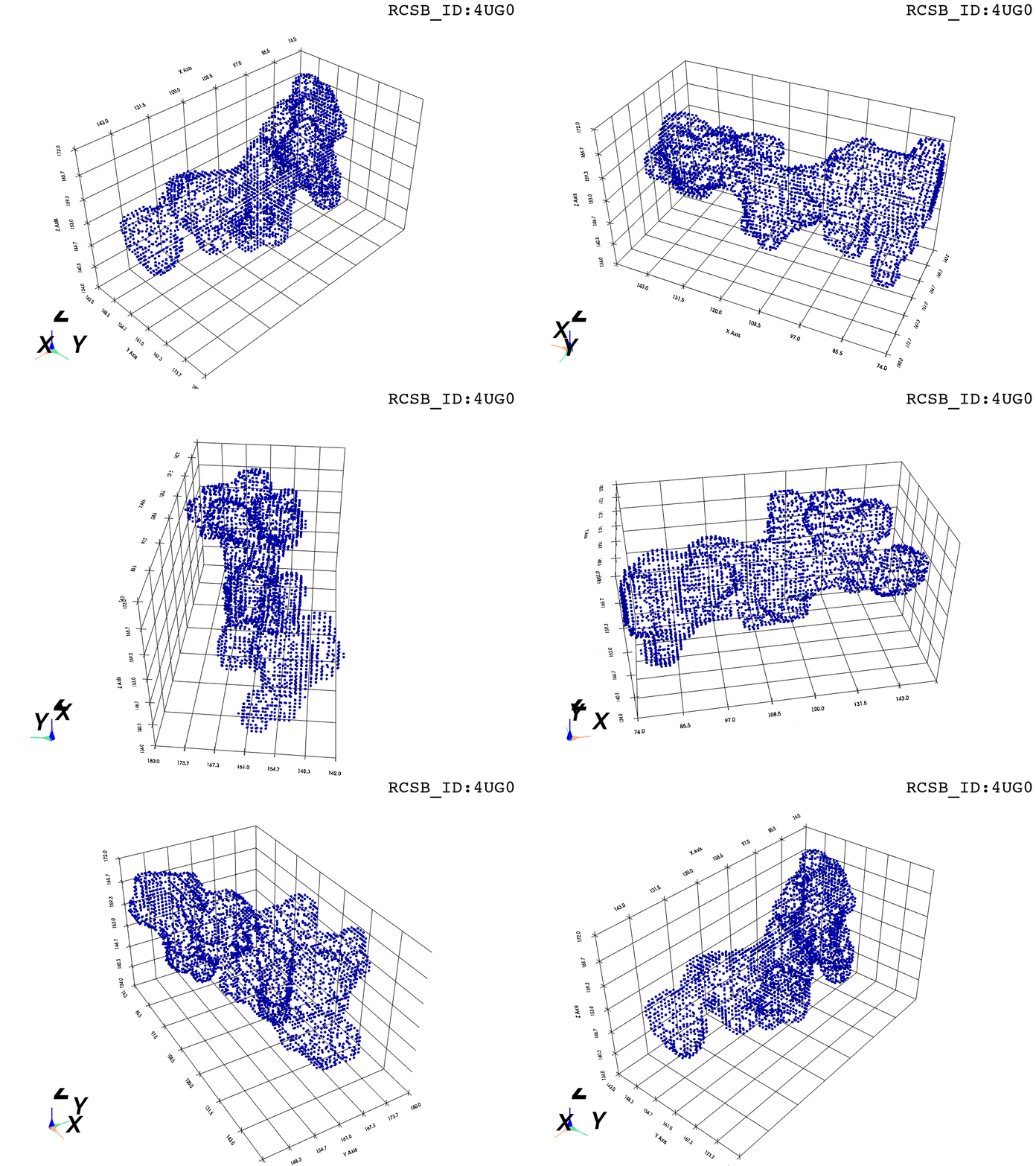
Compare the following representation (Inverted Point Cloud) to the first point cloud: notice that where there previously was an active voxel is now an empty voxel and vice versa. The tubular constellation of active voxels in the center of the bounding box on this inverted grid is the tunnel “space” we are interested in.

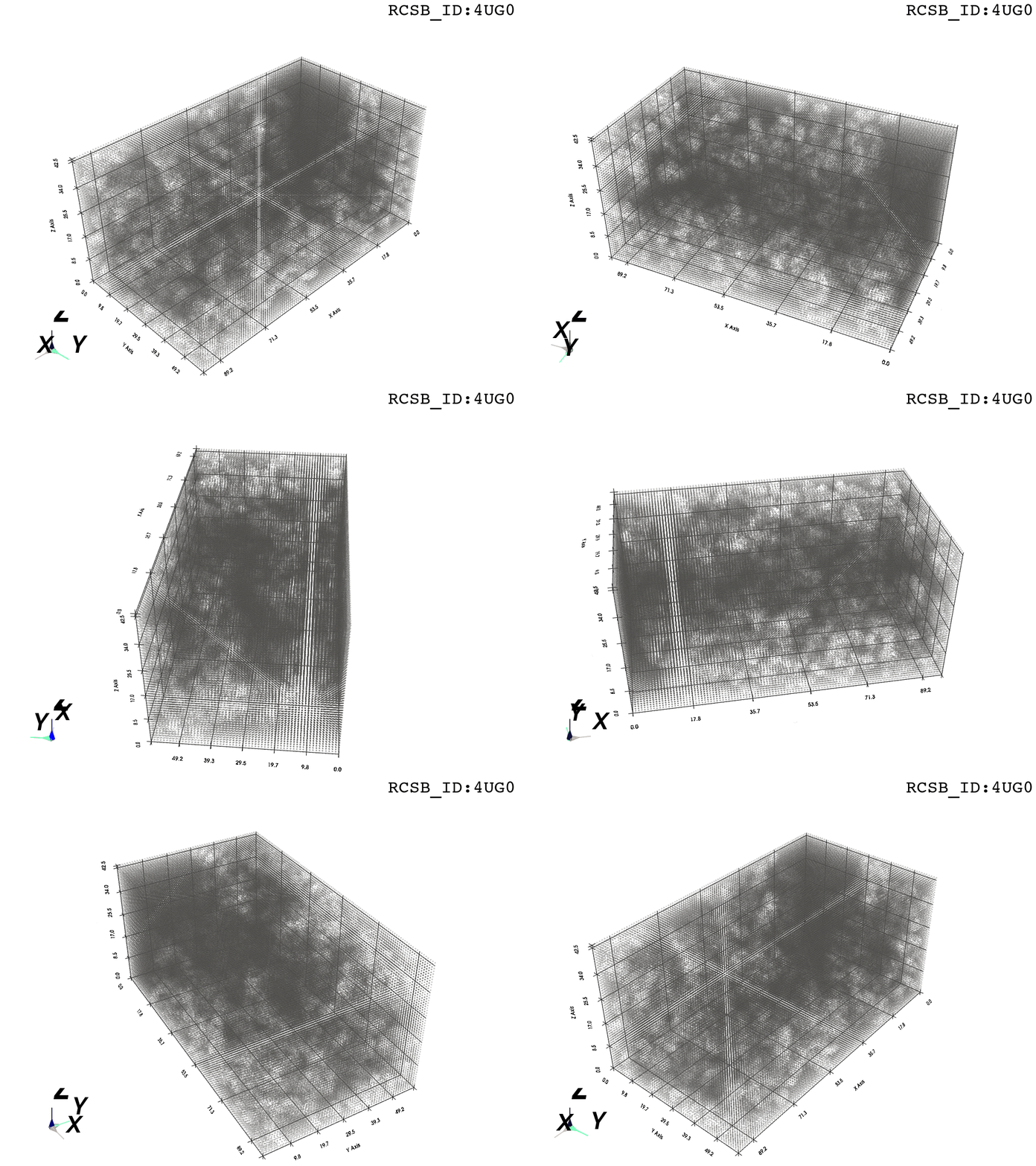
(a) Initial bounding-box point cloud
(b) Inverted point cloud
Figure 1: Pointcloud inversion via a voxel grid.

2. Subcloud Extraction

from sklearn.cluster import DBSCAN
def DBSCAN_capture(
    ptcloud: np.ndarray,
    eps           ,
    min_samples   ,
    metric        : str = "euclidean",
): 

    u_EPSILON     = eps
    u_MIN_SAMPLES = min_samples
    u_METRIC      = metric

    print("Running DBSCAN on {} points. eps={}, min_samples={}, distance_metric={}"
    .format( len(ptcloud), u_EPSILON, u_MIN_SAMPLES, u_METRIC ) ) 

    db     = DBSCAN(eps=eps, min_samples=min_samples, metric=metric).fit(ptcloud) # <-- this is all you need

    labels = db.labels_

    CLUSTERS_CONTAINER = {}
    for point, label in zip(ptcloud, labels):
        if label not in CLUSTERS_CONTAINER:
            CLUSTERS_CONTAINER[label] = []
        CLUSTERS_CONTAINER[label].append(point)

    CLUSTERS_CONTAINER = dict(sorted(CLUSTERS_CONTAINER.items()))
    return db, CLUSTERS_CONTAINER
from sklearn.cluster import DBSCAN
def DBSCAN_pick_largest_cluster(clusters_container:dict[int,list])->np.ndarray:
    DBSCAN_CLUSTER_ID = 0
    for k, v in clusters_container.items():
        if int(k) == -1:
            continue
        elif len(v) > len(clusters_container[DBSCAN_CLUSTER_ID]):
            DBSCAN_CLUSTER_ID = int(k)
    return np.array(clusters_container[DBSCAN_CLUSTER_ID])

Clustering: Having obtained a voxelized representation of the interatomic spaces inside and around the NPET our task is now to extract only the space that corresponds to the NPET. We use DBSCAN.

scikit’s implementation of DBSCAN conveniently lets us retrieve the points from the largest cluster only, which corresponds to the active voxels of NPET space (if we eyeballed our DBSCAN parameters well).

from scikit.cluster import DBSCAN

_u_EPSILON, _u_MIN_SAMPLES, _u_METRIC  = 5.5, 600, 'euclidian'

_, clusters_container   = DBSCAN_capture(inverted_grid, _u_EPSILON, _u_MIN_SAMPLES, _u_METRIC ) 
largest_cluster         = DBSCAN_pick_largest_cluster(clusters_container)

Our 1Å-side grid just happens to be granular enough to accomodate a “correct” separation of clusters for some empirically established values of min_nbrs and epsilon (DBSCAN parameters), where the largest cluster captures the tunnel space.

A possible issue here is “extraneous” clusters merging into the cluster of interest and thereby corrupting its shape. In general this occurs when there are clusters of density that are close enough (within epsilon to the main one to warrant a merge) and simultaneously large enough that they fulfill the min_nbrs parameter. Hence it might be challenging to find the combination of min_nbrs and epsilon that is sensitive enough to capture the main cluster completely and yet discriminating enough to not subsume any adjacent clusters.

In theory, a finer voxel grid (finer – in relationship to the initial coordinates of the general point cloud; sub-angstrom in our case) would make finding the combination of parameters specific to the dataset easier: given that the atom-sphere would be represented by a proprotionally larger number of voxels, the euclidian distance calculation between two voxels would be less sensitive to the change in epsilon.

Partioning the voxel grid further would come at a cost:

  • you would need to rewrite the sphering method for atoms (to account for the the new voxel-size)
  • the computational cost will increase dramatically, the dataset could conceivably stop fitting into memory alltogether.
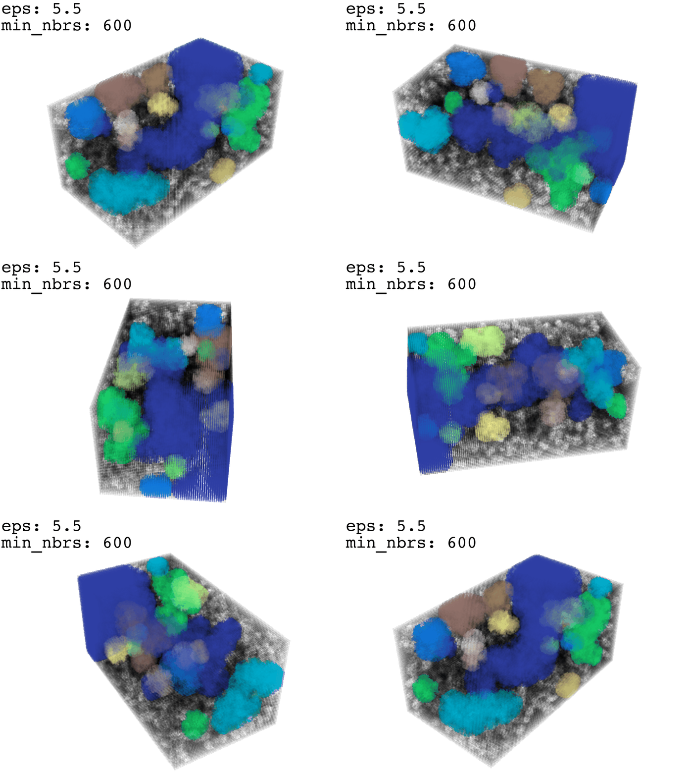
Clusters identified by DBSCAN on the inverted index grid. The largest cluster corresponds to the tunnel space.

I found that this first pass of DBSCAN (eps=\(5.5\), min_nbrs=\(600\)) successfully identifies the largest cluster with the tunnel but generally happens to be conservative in the amount of points that are merged into it. That is, there are still redundant points in this cluster that would make the eventual surface reconstruction spatially overlap with the rRNA and protiens. To “sharpen” this cluster we apply DBSCAN only to its sub-pointcloud and push the eps distance down to \(3\) and min_nbrs to \(123\) (again, “empirically established” values), which happens to be about the lowest parameter values at which any clusters form. This sharpened cluster is what the tesselation (surface reconstruction) will be performed on.

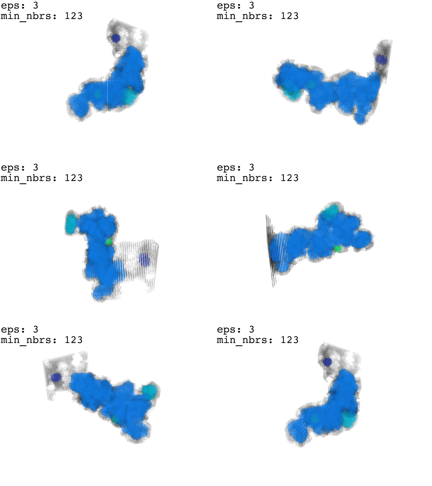
(a) Largest DBSCAN cluster (trimmed from the vestibule side).
(b) Cluster refinement: DBSCAN{e=3,mn=123} result (marine blue) on the largest cluster of DBSCAN{e=5.5,mn=600} (gray)
Figure 2: Second pass of DBSCAN sharpens the cluster to peel off the outer layer of redundant points.

3. Tessellation

Surface points can be extracted by creating an alpha shape over the point cloud and taking only the points that belong to the alpha surface.

import pyvista as pv
import open3d as o3d
import numpy as np

def ptcloud_convex_hull_points(pointcloud: np.ndarray, ALPHA:float, TOLERANCE:float) -> np.ndarray:
    assert pointcloud is not None
    cloud       = pv.PolyData(pointcloud)
    grid        = cloud.delaunay_3d(alpha=ALPHA, tol=TOLERANCE, offset=2, progress_bar=True)
    convex_hull = grid.extract_surface().cast_to_pointset()
    return convex_hull.points

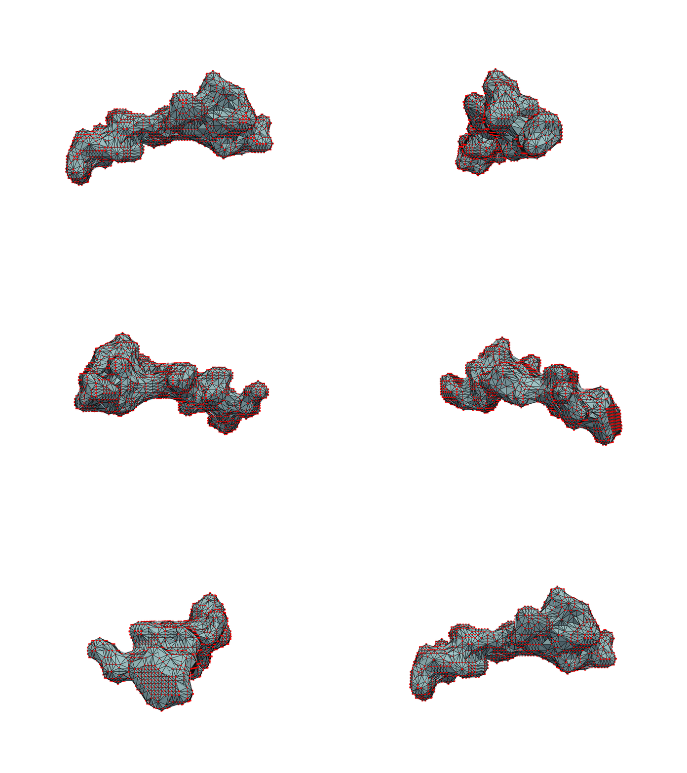
One could content themselves with the alpha shape representation of the NPET geometry and stop here, but it’s easy to notice that the vertice of the polygon (red dots) are distributed unevenly over the surface. This is likely to introduce artifacts and instabilities into further simulations.

(a) Alpha-shape over the pointcloud
(b) Surface points of the point cloud
Figure 3: Alpha shape provides a way to identify surface points.

Normal estimation is done via rolling a tangent plane over the surface points.

import pyvista as pv
import open3d as o3d
import numpy as np

def estimate_normals(convex_hull_surface_pts: np.ndarray, kdtree_radius=None, kdtree_max_nn=None, correction_tangent_planes_n=None): 
    pcd        = o3d.geometry.PointCloud()
    pcd.points = o3d.utility.Vector3dVector(convex_hull_surface_pts)

    pcd.estimate_normals(search_param=o3d.geometry.KDTreeSearchParamHybrid(radius=kdtree_radius, max_nn=kdtree_max_nn) )
    pcd.orient_normals_consistent_tangent_plane(k=correction_tangent_planes_n)

    return pcd

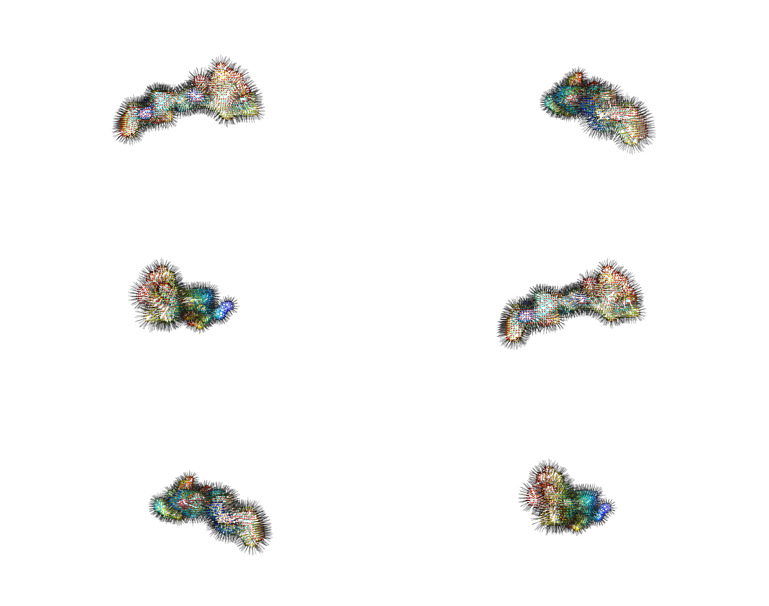
Normals’ orientations are depicted as vectors(black) on each datapoint.

The source is available at https://github.com/mkazhdan/PoissonRecon. For programmability we connect the binary to the pipeline by wrapping it in a python subprocess but one can of course use the binary directly.

The output of the binary is a binary .ply (Stanford Triangle Format) file. For purposes of distribution we also produce an asciii-encoded version of this .ply file side-by-side: some geometry packages are only able to parse the ascii version.

def apply_poisson_reconstruction(surf_estimated_ptcloud_path: str, recon_depth:int=6, recon_pt_weight:int=3):
    import plyfile
    # The documentation can be found at https://www.cs.jhu.edu/~misha/Code/PoissonRecon/Version16.04/ in "PoissonRecon" binary
    command = [
        POISSON_RECON_BIN,
        "--in",
        surf_estimated_ptcloud_path,
        "--out",
        output_path,
        "--depth",
        str(recon_depth),
        "--pointWeight",
        str(recon_pt_weight),
        "--threads 8"
    ]
    process = subprocess.run(command, capture_output=True, text=True)
    if process.returncode == 0:
        print(">>PoissonRecon executed successfully.")
        print(">>Wrote {}".format(output_path))
        # Convert the plyfile to asciii
        data = plyfile.PlyData.read(output_path)
        data.text = True
        ascii_duplicate =output_path.split(".")[0] + "_ascii.ply"
        data.write(ascii_duplicate)
        print(">>Wrote {}".format(ascii_duplicate))
    else:
        print(">>Error:", process.stderr)

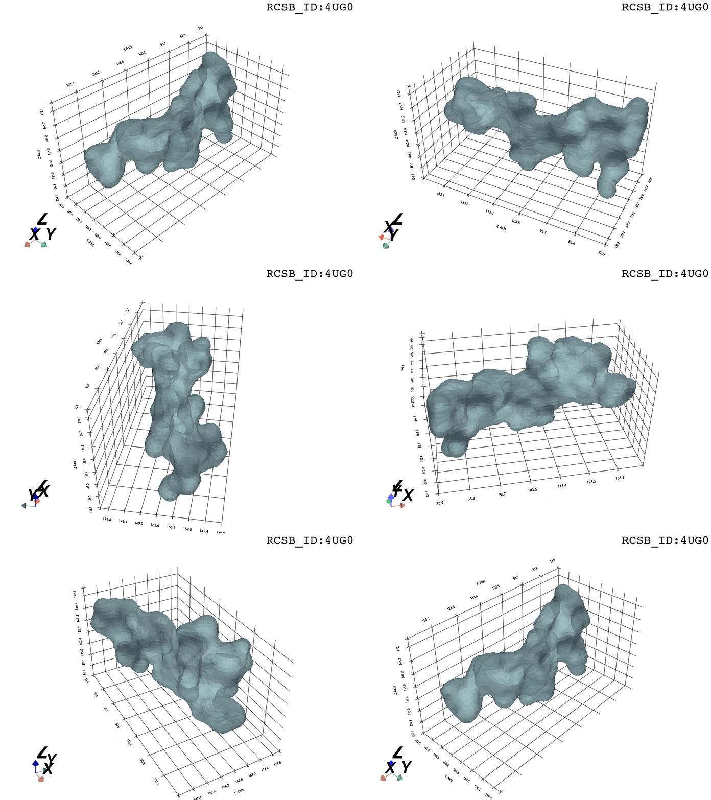
The final NPET surface reconstruction

Now, having refined the largest DBSCAN cluster, we have a pointcloud which faithfully represent the tunnel geometry. To create a watertight mesh from this point cloud we need to prepare the dataset:

  • retrieve only the “surface” points from the pointcloud
  • estimate normals on the surface points (establish data orientation)
d3d_alpha, d3d_tol     = 2, 1

surface_pts = ptcloud_convex_hull_points(coordinates_in_the_original_frame, d3d_alpha,d3d_tol)
pointcloud  = estimate_normals(surface_pts, kdtree_radius=10, kdtree_max_nn=15, correction_tangent_planes_n=10)

The dataset is now ready for surface reconstruction. We reach for Poisson surface reconstruction4 by Kazhdan and Hoppe, a de facto standard in the field.

PR_depth , PR_ptweight = 6, 3
apply_poisson_recon(pointcloud, recon_depth=PR_depth, recon_pt_weight=PR_ptweight)

Result

What you are left with is a smooth polygonal mesh in the .ply format. Below is the illustration of the fidelity of the representation. Folds and depressions can clearly be seen engendered by three proteins surrounding parts of the tunnel (uL22 yellow, uL4 light blue and eL39 magenta). rRNA is not shown.6
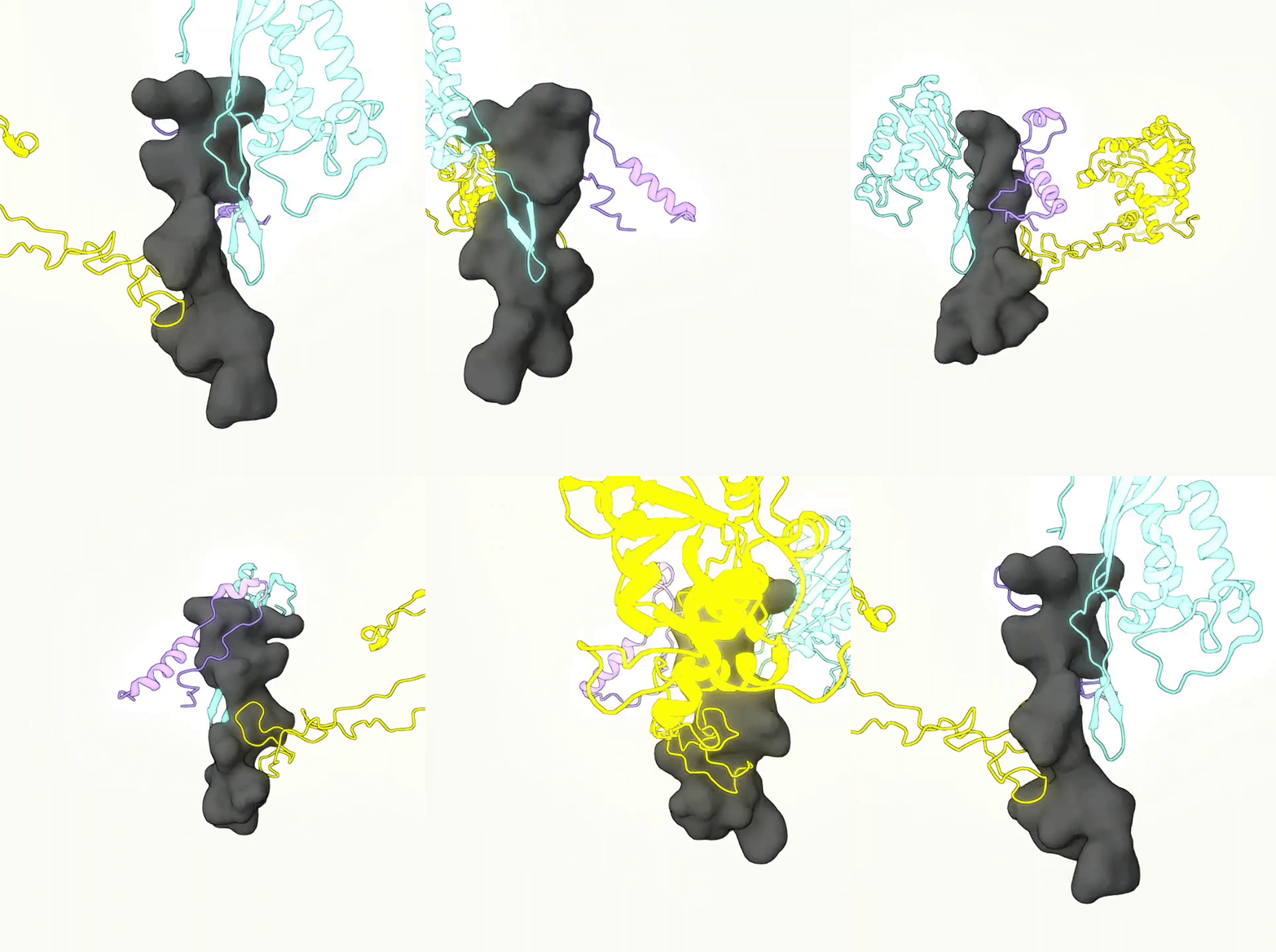
The NPET mesh surrounded by by three ribosome proteins

References

1.
Dao Duc, K. & Song, Y. S. The impact of ribosomal interference, codon usage, and exit tunnel interactions on translation elongation rate variation. PLoS genetics 14, e1007166 (2018).
2.
Dao Duc, K., Batra, S. S., Bhattacharya, N., Cate, J. H. & Song, Y. S. Differences in the path to exit the ribosome across the three domains of life. Nucleic acids research 47, 4198–4210 (2019).
3.
Sehnal, D. et al. MOLE 2.0: Advanced approach for analysis of biomacromolecular channels. Journal of cheminformatics 5, 1–13 (2013).
4.
Kazhdan, M., Bolitho, M. & Hoppe, H. Poisson surface reconstruction. in Proceedings of the fourth eurographics symposium on geometry processing vol. 7 (2006).
5.
Zhou, Q.-Y., Park, J. & Koltun, V. Open3D: A modern library for 3D data processing. arXiv preprint arXiv:1801.09847 (2018).
6.
Sullivan, C. & Kaszynski, A. PyVista: 3D plotting and mesh analysis through a streamlined interface for the visualization toolkit (VTK). Journal of Open Source Software 4, 1450 (2019).