import numpy as np
import scipy as scp
import matplotlib
import matplotlib.pyplot as plt
"figure.figsize"] = (20,20)
plt.rcParams[
= np.array([0,0])
mean = np.array([[0.5, 0.25], [0.25, 0.5]])
cov = scp.stats.multivariate_normal(cov = cov, mean = mean, seed = 1)
distr
= plt.subplots(figsize=(8,8))
fig, ax = ax.imshow([[distr.pdf([i/100,j/100]) for i in range(100,-100,-1)] for j in range(-100,100)], extent=[-1, 1, -1, 1])
im = ax.figure.colorbar(im, ax=ax)
cbar "The pdf of our primal distribution")
plt.title( plt.show()
Introduction
In the context of cryo-EM, many computationally exhaustive methods rely on simpler representations of cryo-EM density maps to overcome their scalability challenges. There are many choices for the form of the simpler representation, such as vectors (Han et al. 2021) or a mixture of Gaussians (Kawabata 2008). In this post, we discuss a format that is probably the simplest and uses a set of points (called a point cloud).
This problem can be formulated in a much more general sense rather than cryo-EM. In this sense, we are given a probability distribution over \(\mathbb{R}^3\) and we want to generate a set of 3D points that represent this distribution. The naive approach for finding such a point cloud is to just sample points from the distribution. Although this approach is guaranteed to find a good representation, it needs many points to cover the distribution evenly. Since methods used in this field can be computationally intensive with cubic or higher time complexity, generating a point cloud that covers the given distribution with a smaller point-cloud size leads to a significant improvement in their runtime.
In this approach, we present two methods for generating a point cloud from a cryo-EM density map or a distribution in general. The first one is based on the Topological Representing Network (TRN) (Martinetz and Schulten 1994) and the second one combines the usage of the Optimal Transport (OT) (Peyré, Cuturi, et al. 2019) theory and a computational geometry object named Centroidal Voronoi Tessellation (CVT).
Data
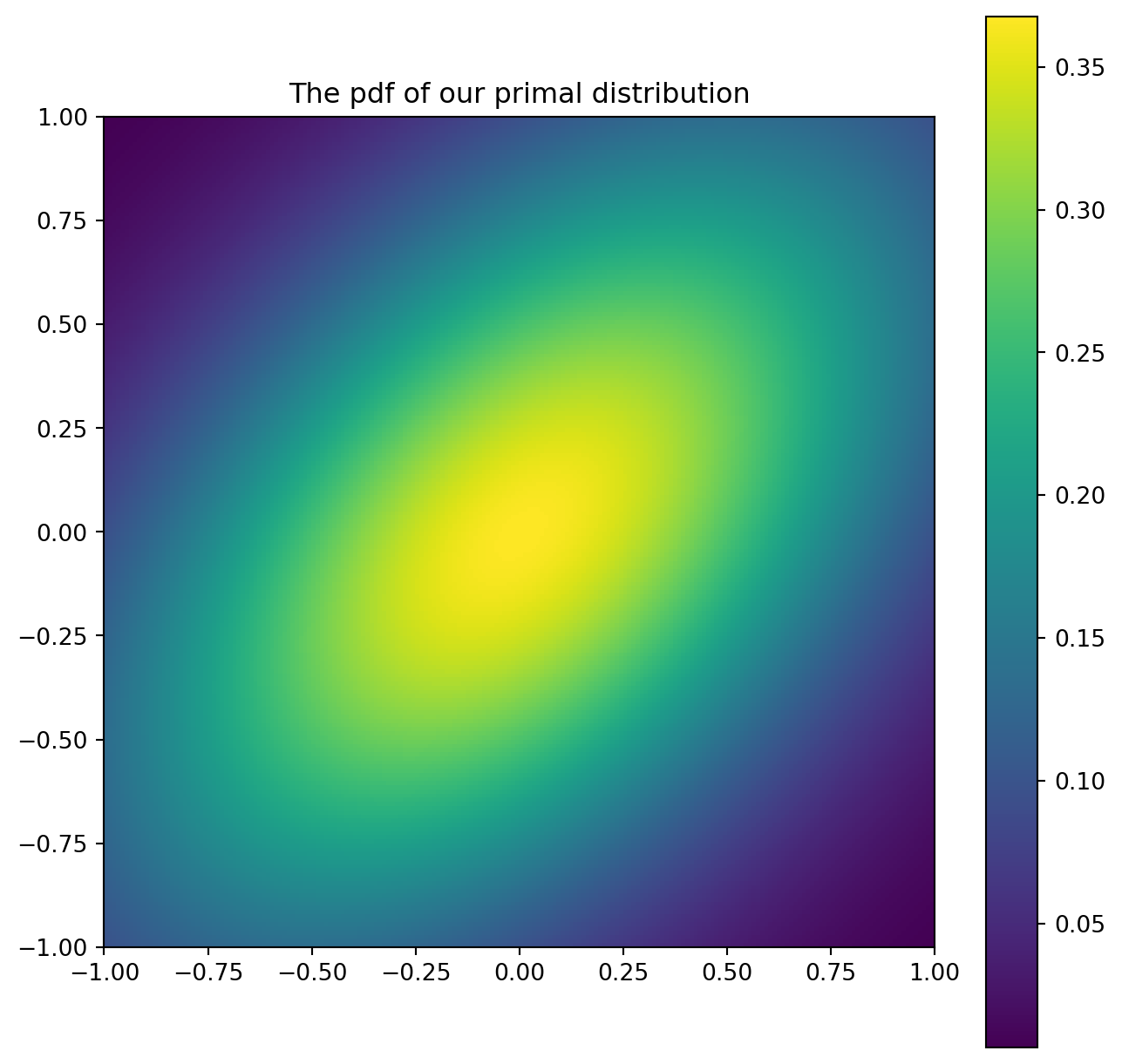
For the sake of simplicity in this post, we assume we are given a primal distribution over \(\mathbb{R}^2\). As an example, we will work on a multivariate Gaussian distribution that it’s domain is limited to \([0, 1]^2\). The following code prepares and illustrates the pdf of the example distribution.
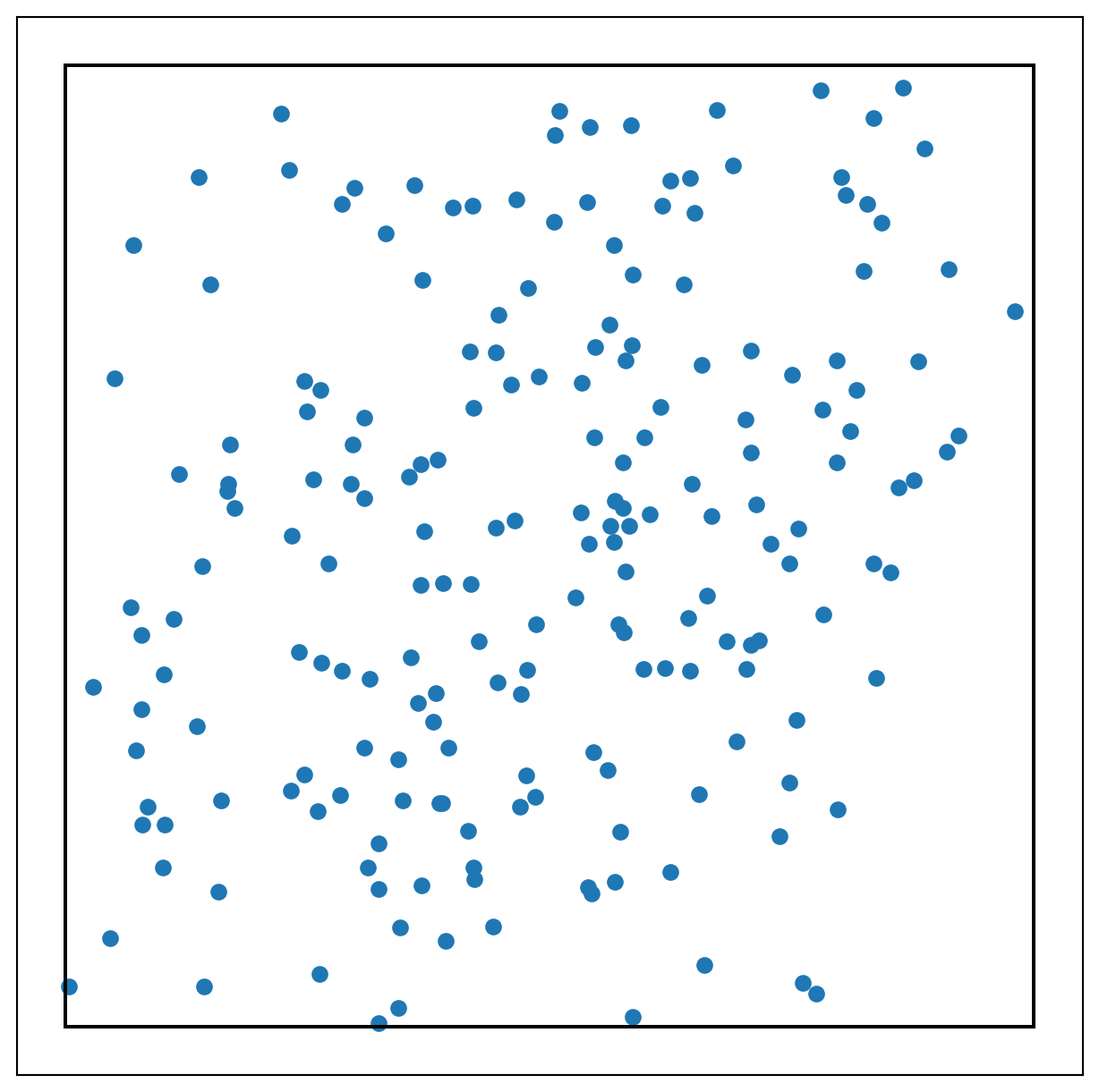
Both of the methods that we are going to cover are iterative methods relying on an initial sample of points. For generating a point cloud with size \(n\), they begin by randomly sampling \(n\) points and refining it over iterations. We use \(n=200\) in our examples.
def sampler(rvs):
while True:
= rvs(1)
sample if abs(sample[0]) > 1 or abs(sample[1]) > 1:
continue
return sample
= []
initial_samples while len(initial_samples) < 200:
= sampler(distr.rvs)
sample list(sample))
initial_samples.append(= np.array(initial_samples)
initial_samples
= list(zip(*initial_samples))
l = list(l[0])
x = list(l[1])
y
= plt.subplots(figsize=(8,8))
fig, ax
ax.scatter(x, y)-1,-1), (-1,1), 'k-')
ax.plot((-1,1), (-1,-1), 'k-')
ax.plot((1,1), (1,-1), 'k-')
ax.plot((-1,1), (1,1), 'k-')
ax.plot((-1.1,1.1)
plt.ylim(-1.1,1.1)
plt.xlim(
plt.xticks([])
plt.yticks([]) plt.show()
Topology Representing Networks (TRN)
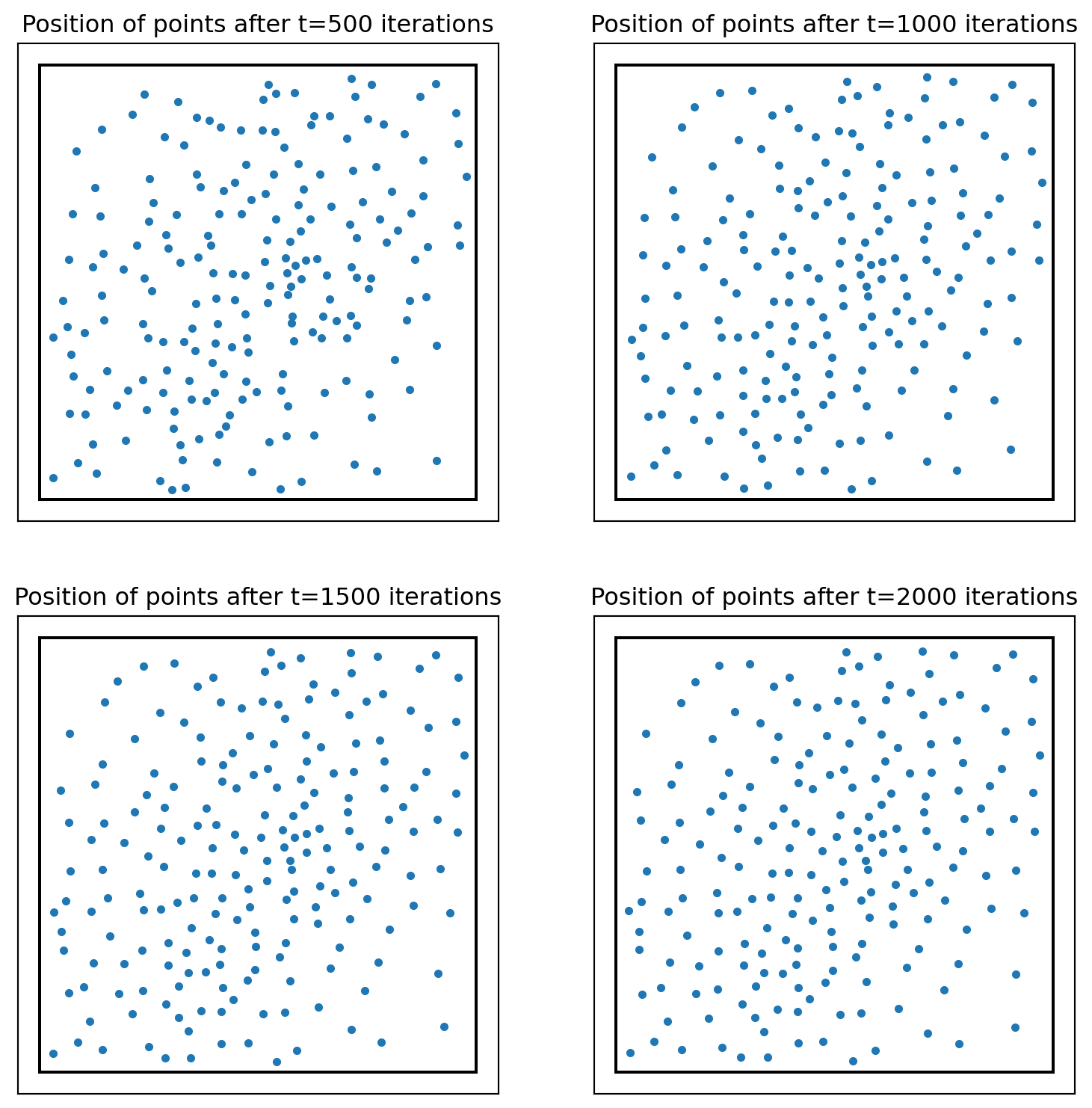
TRN is an iterative method that relies on randomly sampling an initial point cloud \(r_m(0)_{i=1,\dots,n}\) from the given probability distribution \(p\). At each step \(t\), they sample a new point (\(r_t\)) from \(p\) and compute the distance from points in \(r_m(t)\) to \(r_t\) and rank them from zero (closest) to \(n-1\) (called \(k_m\)). Then they update the position of points based on: \[r_m(t+1) = r_m(t) + \epsilon(t)exp(-k_m/\lambda(t))(r_t - r_m(t)),\] \[\epsilon(t) = \epsilon_0(\frac{\epsilon_f}{\epsilon_0})^{t/t_f},\] \[\lambda(t) = \lambda_0(\frac{\lambda_f}{\lambda_0})^{t/t_f}\] These equations are designed in a way that moves points slower as the number of iterations increases.
=0.5
e0=0.05
ef=1
l0=0.5
lf=2000 tf
= plt.subplots(2, 2, figsize=(9.5,9.5))
fig, axs
= initial_samples
r for t in range(tf):
= sampler(distr.rvs)
rt = ((rt - r)**2).sum(1)
dist2 = dist2.argsort()
order = order.argsort().reshape(-1,1)
rank = l0*(lf/l0)**(t/tf)
l = e0*(ef/e0)**(t/tf)
e = r + e*np.exp(-rank/l)*(rt-r)
r
if (t+1)%500 == 0:
= list(zip(*r))
l = list(l[0])
x = list(l[1])
y
= t//500
index //2][index%2].scatter(x, y, s=10)
axs[index//2][index%2].title.set_text('Position of points after t=%d iterations'%(t+1,))
axs[index//2][index%2].plot((-1,-1), (-1,1), 'k-')
axs[index//2][index%2].plot((-1,1), (-1,-1), 'k-')
axs[index//2][index%2].plot((1,1), (1,-1), 'k-')
axs[index//2][index%2].plot((-1,1), (1,1), 'k-')
axs[index-1.1,1.1)
plt.ylim(-1.1,1.1)
plt.xlim(//2][index%2].set_xticks([])
axs[index//2][index%2].set_yticks([])
axs[index plt.show()
Centroidal Vornoi Tessellation (CVT)
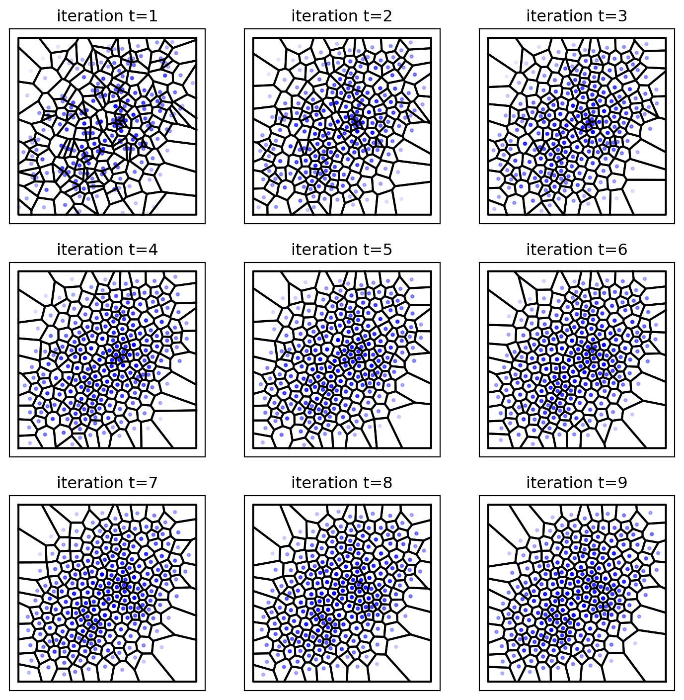
Although TRN is intuitive it doesn’t minimize any specific objective function. Among the metrics that can be for determining the distance between a point cloud and a continuous distribution the semidiscrete Wasserstein distance (based on the Optimal Transport theory (Peyré, Cuturi, et al. 2019)) is of our interest. In other words, we want a point cloud that minimizes the semidiscrete Wasserstein distance to a given primal distribution. One can prove that such a point cloud forms a geometrical object named Centroidal Voronoi Tessellation (CVT) over the distribution. A CVT is a Voronoi diagram generated by a point cloud such that each point is centroid and generator of it’s Voronoi cell. More details about this object will be covered in future posts. Such a tessellation can be computed using Lloyd’s iterations by alternating between computing centroids and Voronoi cells. Unlike TRN this method generated a weighted point cloud.
def in_box(robots, bounding_box):
return np.logical_and(np.logical_and(bounding_box[0] <= robots[:, 0],
0] <= bounding_box[1]),
robots[:, 2] <= robots[:, 1],
np.logical_and(bounding_box[1] <= bounding_box[3]))
robots[:,
def voronoi(robots, bounding_box):
= in_box(robots, bounding_box)
i = robots[i, :]
points_center = np.copy(points_center)
points_left 0] = bounding_box[0] - (points_left[:, 0] - bounding_box[0])
points_left[:, = np.copy(points_center)
points_right 0] = bounding_box[1] + (bounding_box[1] - points_right[:, 0])
points_right[:, = np.copy(points_center)
points_down 1] = bounding_box[2] - (points_down[:, 1] - bounding_box[2])
points_down[:, = np.copy(points_center)
points_up 1] = bounding_box[3] + (bounding_box[3] - points_up[:, 1])
points_up[:, = np.append(points_center,
points
np.append(np.append(points_left,
points_right,=0),
axis
np.append(points_down,
points_up,=0),
axis=0),
axis=0)
axis# Compute Voronoi
= scp.spatial.Voronoi(points)
vor # Filter regions and select corresponding points
= []
regions = [] # we'll need to gather points too
points_to_filter = np.arange(points.shape[0])
ind = np.expand_dims(ind,axis= 1)
ind
for i,region in enumerate(vor.regions): # enumerate the regions
if not region: # nicer to skip the empty region altogether
continue
= True
flag for index in region:
if index == -1:
= False
flag break
else:
= vor.vertices[index, 0]
x = vor.vertices[index, 1]
y if not(bounding_box[0] - eps <= x and x <= bounding_box[1] + eps and
2] - eps <= y and y <= bounding_box[3] + eps):
bounding_box[= False
flag break
if flag:
regions.append(region)
# find the point which lies inside
== i][0,:])
points_to_filter.append(vor.points[vor.point_region
= np.array(points_to_filter)
vor.filtered_points = regions
vor.filtered_regions return vor
def centroid_region(vertices):
= 0
A = 0
C_x = 0
C_y for i in range(len(vertices)):
= distr.pdf(vertices[i])
p += p
A += vertices[i,0] * p
C_x += vertices[i,1] * p
C_y
/= A
C_x /= A
C_y return np.array([[C_x, C_y]]), A
def plot(r,ax):
= voronoi(r, bounding_box)
vor -1.1, 1.1])
ax.set_xlim([-1.1, 1.1])
ax.set_ylim([
for region in vor.filtered_regions:
= vor.vertices[region + [region[0]], :]
vertices 0], vertices[:, 1], 'k-')
ax.plot(vertices[:,
= []
centroids = []
weights
for region in vor.filtered_regions:
= vor.vertices[region + [region[0]], :]
vertices = centroid_region(vertices)
centroid, w list(centroid[0, :]))
centroids.append(
weights.append(w)
0], vor.filtered_points[:, 1], s=5, c='b', alpha=weights/max(weights))
ax.scatter(vor.filtered_points[:,
ax.set_xticks([])
ax.set_yticks([])
= np.asarray(centroids)
centroids return centroids, weights
import sys
= np.array([-1., 1., -1., 1.])
bounding_box = sys.float_info.epsilon
eps = initial_samples
samples = plt.subplots(3,3,figsize=(9,9))
fig, axs for i in range(9):
//3][i%3].title.set_text('iteration t=%d'%(i + 1,))
axs[i= plot(samples,axs[i//3][i%3])
centroids, weights = np.copy(centroids)
samples
plt.show()
More Examples
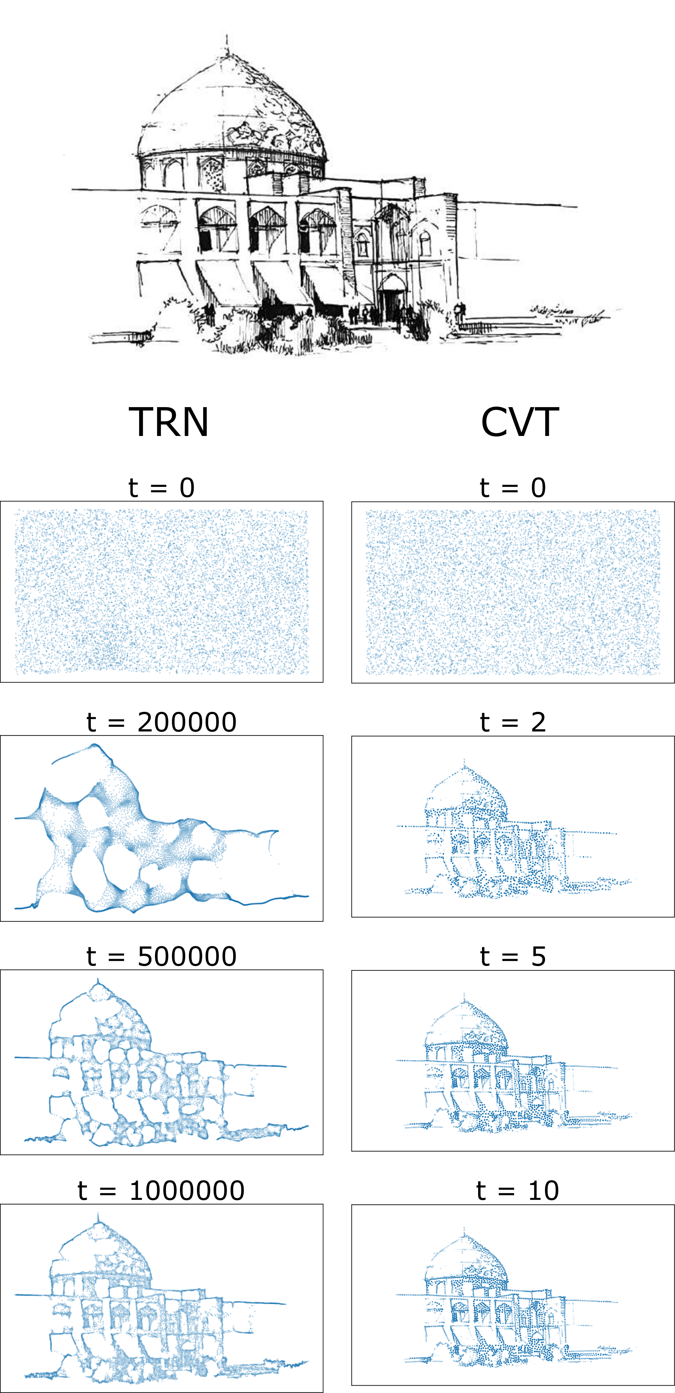
To further examine the effectiveness of these methods, we performed a simulation on a more complex distribution obtained by normalizing the intensities of a sketch of Naqsh-e Jahan Square and \(n=10^5\) points. This image shows the convergence of methods as well as the primal distribution.
Application on Cryo-EM
Both of these methods are easily applicable to a 3D density map. A full implementation of both methods in ChimeraX (the standard visualization tool for cryo-EM) (Pettersen et al. 2021) is in this GitHub repo. TRN was first used in the field of cryo-EM by (Zhang et al. 2021), later on, we used it in our alignment methods Riahi, Zhang, et al. (2023). An example of its performance on cryo-EM density map EMDB:1717 is illustrated below. To the best of our knowledge, no paper has used CVT in the field of cryo-EM yet.