Exploring the relation between cell shape and motility
Cell Morphology
Cell Migration
Differential Geometry
Author
Pavel Buklemishev
Published
October 28, 2024
Background
Cell morphology is an emerging field of biological research that examines the shape, size, and internal structure of cells to describe their state and the processes occurring within them. Today, more and more scientist across the world are investigating visible cellular transformations to predict cellular phenotypes. This research has significant practical implications: understanding specific cellular features characteristic of certain diseases, such as cancer, could lead to new approaches for early detection and classification.
In this work, we will explore aspects of cell motility by analyzing the changing shapes of migrating cells. As a cell moves through space, it reorganizes its membrane, cytosol, and cytoskeletal structures (Mogilner and Oster 1996). For example, past experimental studies show that actin polymerization causes protrusions at the leading edge of a cell, forming specific structures known as lamellipodia and filopodia (Lauffenburger and Horwitz 1996), while cells elongate along the direction they move(SenGupta, Parent, and Bear 2021).
Goals
Our goal is to perform a differential geometry analysis of cellular shape curves to explore the correlation between shape differences and spatial displacement. Using the Riemann Elastic Metric(Li et al. 2023):
\[
g_c^{a, b}(h, k) = a^2 \int_{[0,1]} \langle D_s h, N \rangle \langle D_s k, N \rangle \, ds
+ b^2 \int_{[0,1]} \langle D_s h, T \rangle \langle D_s k, T \rangle \, ds
\]
we can estimate the geodesic distance between two cellular boundary curves to mathematically describe how the cell shape changes over time. To implement this algorithm, we will use the Python Geomstats package.
Dataset
This dataset contains real cell contours obtained via fluorescent microscopy in Professor Prasad’s lab, segmented by Clément Soubrier.
204 directories:
Each directory is named cell_*, representing an individual cell.
Frames:
Subdirectories inside each cell are named frame_*, capturing different time points for that cell.
NumPy Array Objects in Each Frame
centroid.npy: Stores the coordinates of the cell’s centroid.
outline.npy: Contains segmented points as Cartesian coordinates.
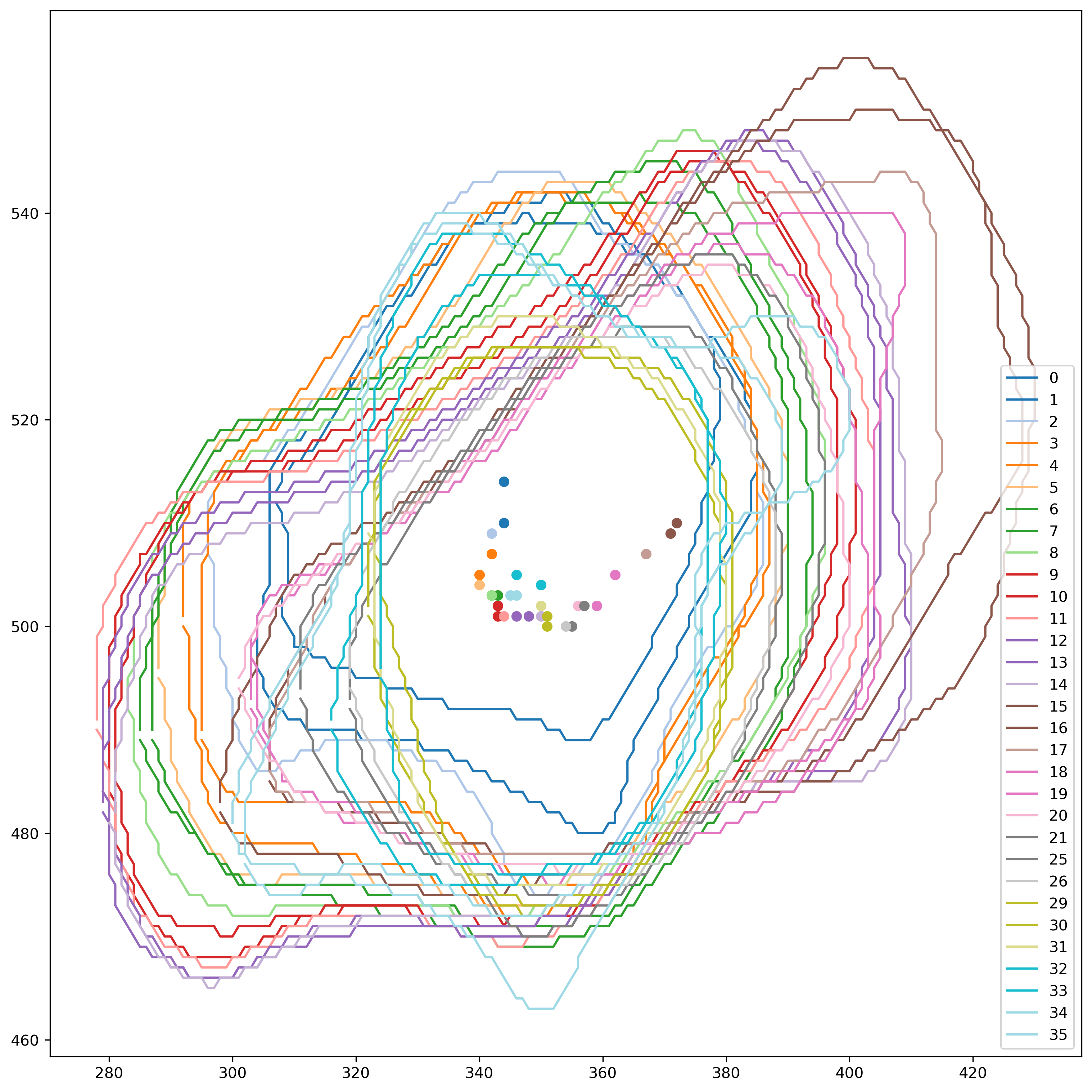
In this section, we provide the code which allows to demonstrate the temporary-spatial cell dynamics. In this particular example we are visualizing the shapes and position of dataset cell №15 Figure 1 which we will be investigated in the project.
Code
import numpy as npimport matplotlib.pyplot as pltimport osfig, ax = plt.subplots(figsize=(10, 10), layout='constrained')N =15number_of_frames =sum(os.path.isdir(os.path.join(f"cells/cell_{N}", entry)) for entry in os.listdir(f"cells/cell_{N}"))colors = plt.cm.tab20(np.linspace(0, 1, number_of_frames))for i inrange(1,number_of_frames+1): time = np.load(f'cells/cell_{N}/frame_{i}/time.npy') border = np.load(f'cells/cell_{N}/frame_{i}/outline.npy') centroid = np.load(f'cells/cell_{N}/frame_{i}/centroid.npy') color = colors[i -1] ax.plot(border[:, 0], border[:, 1], label=time, color=color) ax.scatter(centroid[0], centroid[1], color=color)plt.legend() plt.savefig(f"single_cell_{N}.png", dpi=300, bbox_inches='tight')
Figure 1: The cell #15 in different time moments. The colored curves visualize the cell shape in different time moments, the colored dots are centroids. Each color corresponds to a certain time moment which is shown in the legend.
Li, Wanxin, Ashok Prasad, Nina Miolane, and Khanh Dao Duc. 2023. “Using a Riemannian Elastic Metric for Statistical Analysis of Tumor Cell Shape Heterogeneity.” In Geometric Science of Information, edited by Frank Nielsen and Frédéric Barbaresco, 583–92. Cham: Springer Nature Switzerland.
SenGupta, Shuvasree, Carole A. Parent, and James E. Bear. 2021. “The Principles of Directed Cell Migration.”Nature Reviews Molecular Cell Biology 22 (8): 529–47. https://doi.org/10.1038/s41580-021-00366-6.