This page introduces basic concepts of elastic metric, square root velocity metric, geodesic distance and Fréchet mean associated with it.
Definition
The family of elastic metrics, introduced by Mio et al. (Mio, Srivastava, and Joshi 2007), can be defined over the space \(\mathcal{C}\) of smooth parametrized curves \(c:[0,1]\mapsto \mathbb{R}^2\) with nowhere-vanishing derivative. With \(a,b>0\) denoting the parameters of the family, one associates with every curve \(c \in \mathcal{C}\) an inner product \(g^{a, b}_c\) over the tangent space \(T_c{\mathcal{C}}\), given by Bauer et al. (2014); Needham and Kurtek (2020),
\[g^{a, b}_c(h, k) = a^2\int_{[0,1]}\langle D_sh, N\rangle\langle D_sk, N\rangle ds + b^2 \int_{[0,1]}\langle D_sh, T\rangle\langle D_sk, T\rangle ds, \tag{1}\]
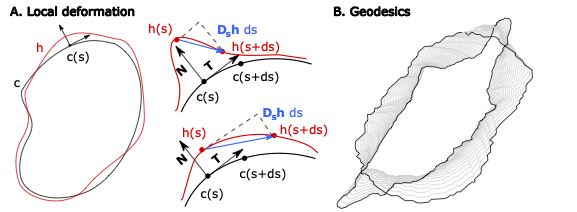
where \(h,k\) are two curve deformations in the tangent space \(T_c{\mathcal{C}}\), that can also be considered as planar curves (Mio, Srivastava, and Joshi 2007); \(<,>\) is the Euclidean inner-product in \(\mathbb{R}^2\), \(D_s = \frac{1}{||c'(s)||}\frac{d}{ds}\), is a differential operator with respect to the arc length \(s\), and \(N\) and \(T\) respectively are the local unit normal and tangent from a moving frame associated with \(c\).
Intuitively, elements in \(T_c{\mathcal{C}}\) represent infinitesimal deformations of \(c\), and \(g^{a, b}_c\) quantifies the magnitude of these deformations, with the two factors \(a\) and \(b\) that can be interpreted as weights penalizing the cost of bending (for \(a\)) and stretching (for \(b\)) the curve \(c\).
In Figure 1.A, we illustrate how the metric can be interpreted for a local deformation \(h\) of \(c\): As we project the derivative of \(h\) (with respect to its arc length) along the tangent and normal vectors of the reference frame associated with \(c\), increasing the bending in \(h\) results in a relatively higher contribution from the normal component, and thus the integral weighted by \(a^2\), according to Equation 1. Similarly, stretching increases the contribution from the tangent component, and the integral weighted by \(b^2\). In the case that \((a,b)=(1,1/2)\), the elastic metric is called Square Root Velocity metric, as it allows in practice for an efficient evaluation (Srivastava et al. 2010; Le Brigant 2019).

Geodesic distance
As a Riemaniann metric (Mio, Srivastava, and Joshi 2007; Srivastava et al. 2010), the elastic metric yields a geodesic distance over \(\mathcal{C}\): For two curves \(c_0\) and \(c_1\) and a regular parameterized path \(\alpha:[0,1] \mapsto \mathcal{C}\) such that \(\alpha(0)=c_0\) and \(\alpha(1)=c_1\), the length of \(\alpha\), associated with the elastic metric \(g^{a,b}\) is given by \[ L^{a,b}[\alpha] = \int_0^1 g^{a,b}_{\alpha(t)} (\alpha'(t),\alpha'(t))^{1/2}dt, \tag{2}\] and the geodesic distance between \(c_0\) and \(c_1\) is \[ d^{a,b}(c_0,c_1) = \inf_{\alpha:[0,1] \mapsto \mathcal{C} \ | \ \alpha(0)=c_0 \ ; \ \alpha(1)=c_1} L^{a,b}[\alpha]. \tag{3}\] Figure 1.B illustrates the shortest path joining two cell shapes using the elastic metric.
An approximation of the geodesic distance associated with the elastic metric \(g^{a,b}\) can be computed as a pull-back of the linear metric: Upon applying a transformation that maps the geodesic associated with \(g^{a, b}\) into a straight line, the geodesic distance is equal to the \(\mathcal{L}^2\) distance between the two transformed curves (Needham and Kurtek 2020). While the procedure to construct the mapping can be numerically unstable (Bauer et al. 2014; Needham and Kurtek 2020), it is simple for the SRV, with the geodesic distance being the \(\mathcal{L}^2\) distance obtained upon representing the curve by its speed, renormalized by the square root of its norm as \(q(c) = \dot{c}/\sqrt{\lvert \dot{c} \rvert}\) (Bauer et al. 2022).
Fréchet mean
With the space of curves equipped with this distance, the so-called Fréchet mean of \(n\) curves \((c_1,\ldots,c_n)\) (Miolane et al. 2020) is defined as \[ \bar{c} = \underset{c \in \mathcal{C}}{\text{argmin}} \sum_{i=1}^n (d^{a,b}(c,c_i))^2. \tag{4}\]