Code
import matplotlib.pyplot as plt
import torch.optim as optim
import torch
from torch import nn
from torchvision.io import read_image
import torch.nn.functional as FPyTorch Implementation of Benamou-Brenier Formulation
December 16, 2024
In this blog post, let us continue from the previous blog post on defining the convex formulation of optimal mass transport (OMT). Specifically, let us look upon the need for application of OMT for interpolation of shapes and learn to implement Benamou-Brenier’s formulation of OMT in python. The problem is essentially a PDE optimization process and hence the numerical solution is expensive. The aglorithm used here is based on an efficient method as described in (Haber, Rehman, and Tannenbaum (2010)). It relies on augmented Lagrangian approach to efficiently solve the constrained optimization. Also, the use of graphics processing unit (GPU) has been evident in accelerating the computation time. (Rehman et al. (2009)) Hence, PyTorch is used for programming the problem here, as it is an excellent easy to use scientific computing framework with the feature of automatic differentiation (Neidinger (2010)) accelerated by GPUs for tensor operations.
The Benamou-Brenier formulation (Benamou and Brenier (2000)) is used, which interprets it as a fluid flow problem. This approach finds the path of continual mass transfer such that minimal “kinetic energy” needed to transform from one state to another.
The Benamou-Brenier formulation considers a probability density \(\rho(x, t)\) evolving over time \(t \in [0, 1]\) from an initial distribution \(\rho_0\) to a final distribution \(\rho_1\). The goal is to find a velocity field \(v(x, t)\) that minimizes the action, or “kinetic energy” cost:
\[ \min_{\rho, v} \int_0^1 \int_X \frac{1}{2} \|v(x, t)\|^2 \rho(x, t) \, dx \, dt, \]
subject to the continuity equation:
\[ \frac{\partial \rho}{\partial t} + \nabla \cdot (\rho v) = 0, \]
which ensures mass conservation from \(\rho_0\) to \(\rho_1\).
The problem is reposed in terms of momentum in x and y respectively as \(m_x = \rho v_x\) and \(m_y = \rho v_y\) as in (Haber, Rehman, and Tannenbaum (2010)). Staggered grid is used for \(m_x\), \(m_y\), and \(\rho\) to stabilize non physical checkerboard instability.
So, the problem is rewritten as:
\[ \min_{m} \int_0^1 \int_{\Omega} \frac{1}{\rho} (m_x^2 + m_y^2) \, dx \, dt, \]
such that
\[ \Delta_x m_x + \Delta_y m_y + \Delta_t \rho = 0, \]
where \(\rho\)(x,y,0) = Image at time 0, and \(\rho\)(x,y,1) = Image at time 1.
Formulating this constrained optimization problem into a KKT problem by Augmented Lagrangian method (Nocedal and Wright (1999)) which is then optimized by Adam’s stochastic gradient descent optimization. (Kingma (2014))
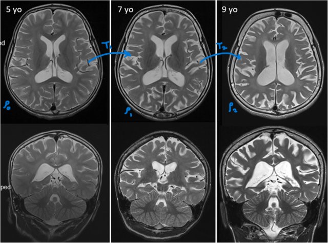
Let us take the MRI image samples (Figure 1) of the vertical and horizontal cross-sections a kid’s brain at the age of 5 years, 7 years and 9 years, as shared by (Bastos et al. (2020)). What if we did not have the MRI scans when the kid was 7 year old? Specifically, if the kid has a disease. If we have an interpolation technique, we can use the scans at the ages 5 and 9 years and look at the sequence of interpolated scans to study which part of brain is under compression and gauge how it affected over time.

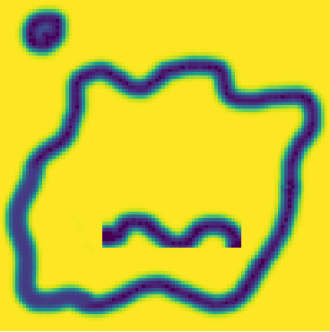
The popular interpolation linear interpolation or any polynomial interpolation is not the best choice in such a case. To study the concept and learn why, let us take a toy case of aging cell. Essentially to generate the interpolation of the shape of a living cell from the images of a young and healthy cell to an old deformed cell.


The basic and most simple method of interpolation is linear interpolation. It is a commonly used technique for generating intermediate images between two given images. It assumes a linear blend of pixel intensities over the interpolation parameter ‘t’, which is time. Mathematically, the equation of the interpolant(\(I_t\)) is given by:
\[ I_t = (1 - t) I_0 + t I_1, \] where \(I_0\) is the image at time 0 and \(I_1\) is the image at time 1.

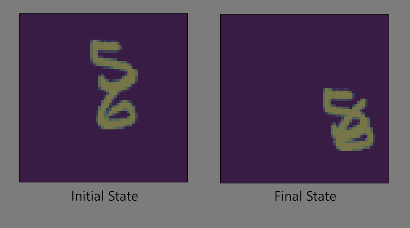
The Figure 3 shows the interpolation of the images of the toy cell when it is healthy and when it is old. It can be seen that what essentially happens is a smooth transition between the two images by linearly interpolating the intensity values of each pixel independently. The transform in shape is not something we see in real life. It is not really a physical transformation. The masses/pixels do not really transport in spatial domain, rather they teleport. This kind of interpolation is hence quite often not beneficial. In the case of MRI scans, Figure 4 shows how the linearly interpolated shape at different ages do not make sense physically. Let us implement an OMT based interpolation on a to a toy problem, whose initial and final images are randomly sampled from MNIST digits, can be seen in Figure 5.


The most import library, here, is torch as it has the ability to perform automatic differentiation and GPU accelerated tensor operations. Torchvision is required for additional image operations and matplotlib for plots.
class omtFD(nn.Module):
    def __init__(self, n1, n2, n3, bs=1):
        super().__init__()
        self.n1 = n1
        self.n2 = n2
        self.n3 = n3
        self.bs = bs

        self.m1 = nn.Parameter(torch.zeros(bs, 1, n1 - 1, n2, n3))
        self.m2 = nn.Parameter(torch.zeros(bs, 1, n1, n2 - 1, n3))
        self.rho = nn.Parameter(torch.zeros(bs, 1, n1, n2, n3 - 1) - 3)

    def OMTconstraintMF(self, I1, I2):
        dx, dy, dt = 1 / self.n1, 1 / self.n2, 1 / self.n3

        ox = torch.zeros(self.bs, 1, 1, self.n2, self.n3).to(self.rho.device)
        oy = torch.zeros(self.bs, 1, self.n1, 1, self.n3).to(self.rho.device)

        I1 = I1.unsqueeze(-1)
        I2 = I2.unsqueeze(-1)
        rhop = torch.exp(self.rho)

        # Add I1 and I2 to rho
        rhoBC = torch.cat((I1, rhop, I2), dim=-1)
        m1BC = torch.cat((ox, self.m1, ox), dim=-3)
        m2BC = torch.cat((oy, self.m2, oy), dim=-2)

        # Compute the Div
        m1x = (m1BC[:, :, :-1, :, :] - m1BC[:, :, 1:, :, :]) / dx
        m2y = (m2BC[:, :, :, :-1, :] - m2BC[:, :, :, 1:, :]) / dy
        rhot = (rhoBC[:, :, :, :, :-1] - rhoBC[:, :, :, :, 1:]) / dt
        return m1x + m2y + rhot

    def OMTgradRho(self, I1, I2):
        I1 = I1.unsqueeze(-1)
        I2 = I2.unsqueeze(-1)

        # Add I1 and I2 to rho
        rhop = torch.exp(self.rho)
        rhoBC = torch.cat((I1, rhop, I2), dim=-1)
        rhox = (rhoBC[:, :, :-1, :, :] - rhoBC[:, :, 1:, :, :])
        rhoy = (rhoBC[:, :, :, :-1, :] - rhoBC[:, :, :, 1:, :])
        rhot = (rhoBC[:, :, :, :, :-1] - rhoBC[:, :, :, :, 1:])

        return rhox, rhoy, rhot

    def OMTobjfunMF(self, I1, I2):
        I1 = I1.unsqueeze(-1)
        I2 = I2.unsqueeze(-1)

        rhop = torch.exp(self.rho)

        ox = torch.zeros(self.bs, 1, 1, self.n2, self.n3).to(self.rho.device)
        oy = torch.zeros(self.bs, 1, self.n1, 1, self.n3).to(self.rho.device)

        # Add I1 and I2 to rho
        rhoBC = torch.cat((I1, rhop, I2), dim=-1)
        m1BC = torch.cat((ox, self.m1, ox), dim=-3)
        m2BC = torch.cat((oy, self.m2, oy), dim=-2)

        # Average quantities to cell center
        m1c = (m1BC[:, :, :-1, :, :] + m1BC[:, :, 1:, :, :]) / 2
        m2c = (m2BC[:, :, :, :-1, :] + m2BC[:, :, :, 1:, :]) / 2
        rhoc = (rhoBC[:, :, :, :, :-1] + rhoBC[:, :, :, :, 1:]) / 2

        f = ((m1c ** 2 + m2c ** 2) / rhoc).mean()
        return f
This class models the dynamics of mass transport with momentum and density fields while ensuring mass conservation via the continuity equation. The learnable parameters defined here are \(m_1\), \(m_2\), and \(\rho\). The specific class functions are OMTconstraintMF, OMTgradRho, and OMTobjfunMF. A common line you can notice is rhop = torch.exp(self.rho), which ensures that rhop is used instead of rho so as to let only positive values to the PDE system so as to conserve the convexity of optimization. OMTconstraintMF calculates the residual of mass conservation by first order finite difference, which is later denoted as constraint(c). OMTgradRho calculates the gradients of the density, which is denoted by rhop. OMTobjfunMF calculates the objective functional (f) which is the kinetic energy as per Benamou-Brenier’s formulation. In this function, to control checkerboard oscillations, the variables are calculated at cell centres.
def LearnOMT(x0, x1, nt=20, device='cpu'):
    t = torch.linspace(0, 1, nt)

    eps = 1e-2

    I1_min = x0.min()
    I2_min = x1.min()
    I1_mean = (x0 - I1_min + eps).mean()
    I2_mean = (x1 - I2_min + eps).mean()

    I1 = (x0 - I1_min + eps) / I1_mean
    I2 = (x1 - I2_min + eps) / I2_mean

    bs = I1.shape[0]
    ch = I1.shape[1]
    n1 = I1.shape[2]
    n2 = I1.shape[3]
    n3 = nt

    omt = omtFD(n1, n2, n3, bs=bs * ch).to(device)

    # input shape for omt: (bs, 1, nx, ny)
    # final output shape for omt: (bs, 1, nx, ny, nt)

    I1 = I1.reshape([bs * ch, 1, n1, n2])
    I2 = I2.reshape([bs * ch, 1, n1, n2])

    optimizer = optim.Adam(omt.parameters(), lr=1e-2)

    num_epochs = 1000  # with incomplete optimization you do not see the transport, rather it appears as one dims and the other brightens up
    opt_iter = 20
    torch.autograd.set_detect_anomaly(True)

    # Train the model
    mu = 1e-2
    delta = 1e-1

    # initialize lagrange multiplier
    p = torch.zeros(n1, n2, n3).to(device)
    for epoch in range(num_epochs):
        # Optimization iterations for fixed p
        for jj in range(opt_iter):
            # Zero the parameter gradients
            optimizer.zero_grad()

            # function evaluation
            f = omt.OMTobjfunMF(I1, I2)
            # Constraint
            c = omt.OMTconstraintMF(I1, I2)

            const = -(p * c).mean() + 0.5 * mu * (c ** 2).mean()

            loss = f + const

            # Backward pass and optimize
            loss.backward()
            torch.nn.utils.clip_grad_value_(omt.parameters(), clip_value=0.5)
            optimizer.step()

        #print('f:', f.item(), '\tconst:', const.item())

        # Update Lagrange multiplier
        with torch.no_grad():
            p = p - delta * mu * c

    rho = omt.rho.detach()
    rhop = torch.exp(rho)

    # Add I1 and I2 to rho
    rhop = torch.cat((I1.unsqueeze(-1), rhop, I2.unsqueeze(-1)), dim=-1)
    rhop = rhop.reshape([bs, ch, n1, n2, n3 + 1])
    rhop = rhop * I1_mean - eps + I1_min  # assuming mass of x0 = mass of x1
    rhop = rhop.detach()   # shape of rhop: (bs, ch, nx, ny, nt+1) includes x0, "nt-1" timesteps, x1

    return rhop
This module starts with normalizations to match the masses of two images and add a background mass. The input tensors x0 and x1 (representing initial and final states) needs to have positive values and scale them to have a mean of 1. This ensures numerical stability during the optimization. The Adam optimizer is set up to train the parameters of the omtFD class.
The training hyperparameters are defined: num_epochs (the number of optimization epochs), opt_iter (the number of inner iterations per epoch), and mu and delta (regularization parameters for the Lagrange multiplier). The Lagrange multiplier p is initialized to enforce the mass conservation constraint. For each epoch, the following steps are performed for opt_iter iterations:
Output Density Interpolation: The optimized density field rho is extracted from the model and exponentiated to compute the final density rhop. The initial and final states (I1 and I2) are concatenated with rhop to include all intermediate densities, forming the complete transport trajectory. The density trajectory rhop is rescaled back to the original input scale and format, ensuring mass conservation. The interpolated density trajectory rhop is returned, with a shape of (batch_size, channels, n1, n2, nt+1). This includes the initial state (x0), the intermediate densities, and the final state (x1).
device = 'cuda:0' # default: 'cpu'

x0 = torch.load('x0.pt')
x1 = torch.load('x1.pt')
# shape of x0 and x1 = [:,:]

size_img = 64
x0 = F.interpolate(x0.unsqueeze(0).unsqueeze(0), size = [size_img,size_img])
x1 = F.interpolate(x1.unsqueeze(0).unsqueeze(0), size = [size_img,size_img])

x0 = x0.to(device)
x1 = x1.to(device)

OMTInterpolation = LearnOMT(x0, x1, nt=10, device = device)
# shape of Interpolation = [|B|,|C|,|X|,|Y|,|T|]OMTInterpolation = OMTInterpolation[0,0].detach().cpu().numpy()
x0 = x0[0,0].unsqueeze(-1)
x1 = x1[0,0].unsqueeze(-1)
Frac = torch.linspace(0,1,OMTInterpolation.shape[-1])
Frac = Frac.unsqueeze(0).unsqueeze(0)
# Linear Interpolation
LinearInt = x1*Frac + (1-Frac)*x0
LinearInt = LinearInt.detach().cpu().numpy()# shape of Interpolation = [|B|,|C|,|X|,|Y|,|T|]
fig, ax = plt.subplots(nrows=2, ncols=OMTInterpolation.shape[-1], figsize=(50, 5))
for i in range(OMTInterpolation.shape[-1]):
ax[0, i].imshow(LinearInt[:, :, i])
ax[0, i].axis('off')
ax[1, i].imshow(OMTInterpolation[:, :, i])
ax[1, i].axis('off')
ax[0,0].set_title('Linear Interpolation', loc='left')
ax[1,0].set_title('OMT Interpolation', loc='left')
plt.show()
The application of Benamou-Brenier’s optimal mass transport (OMT) to model the shape progression demonstrates the power of combining mathematical rigor with modern computational tools. By leveraging the augmented Lagrangian method for efficient PDE-constrained optimization and the GPU acceleration capabilities of PyTorch, we achieved a computationally viable approach to interpolating MRI images across time. This study highlights the potential of OMT in predicting missing temporal states in medical imaging, such as generating plausible MRI scans at intermediate ages. Interpolation result can be observed in Figure 6. The OMT interpolation looks very physical. Such advancements can contribute significantly to understanding shape morphing and interpolation. Future work could explore extending this approach to complex 2D shapes or 3D volumes like those in MRI scans, integrating other imaging modalities, and refining the method to address even larger datasets.